The second project has two major components: web scraping (BeautifulSoup, Selenium) and linear regression (ScikitLearn, StatsModels). My topic came from previous experience as a geomorphologist and costal engineerer: is it possible to predict sediment concentration in the lower Mississippi River using upstream hydrological data?

Motivation: save the sinking coasts with sediments

Apart from water, rivers carry another critical component that shapes the surface of this planet: sediments. Think about the Nile River. The rich soil brought by annual flooding nurtured one of the earliest civilization. The healthy connection between rivers and their floodplains is essential to the productivity and well-being of the whole eco-system, humans included. However, modern rivers are often leveed for management and flood-protection reasons, such as the Mississippi River. As a result, most of the sediments carried by the Mississippi River, more than 200 million metric tons per year, are directly flushed into the deep gulf of Mexico, while the delta wetlands are starved from the material to build land and sinking into the rising sea.

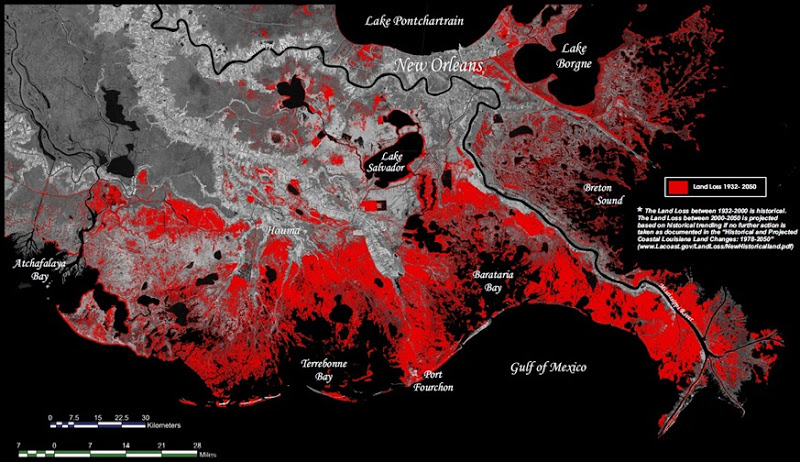
The motivation of this project came from recent initiatives to implement controled sediment diversions to build land in the Mississippi Delta. While these diversions bring land-building sediments, they also indroduce great volume of fresh water, which could have negative impact on the brackish ecosystem. To address this concern, the best operating scheme is to open the diversion during the time period that the river has high sediment concentration.

For this project, I will be look at using linear regression to predict the sediment concentration in the lower Mississippi, using commonly available hydrological data (discharge, stage) from upstream stations.

Webscraping from USGS water data

Hydrological data are available from United States Geological Survey (USGS water data). The primary tool was BeautifulSoup, as many tables cannot be read with python pandas directly. Some pages contained dynamic table with Java script, and required Selenium to load completely. I followed these steps to get the stations I needed for this project:

• Use keyword search to get a list of the stations on the tributary of interest:

• For each station in the lists, follow the URL to get data inventory for daily averaged values

• Determine which station has desired data type and range, then download data file using provided download link

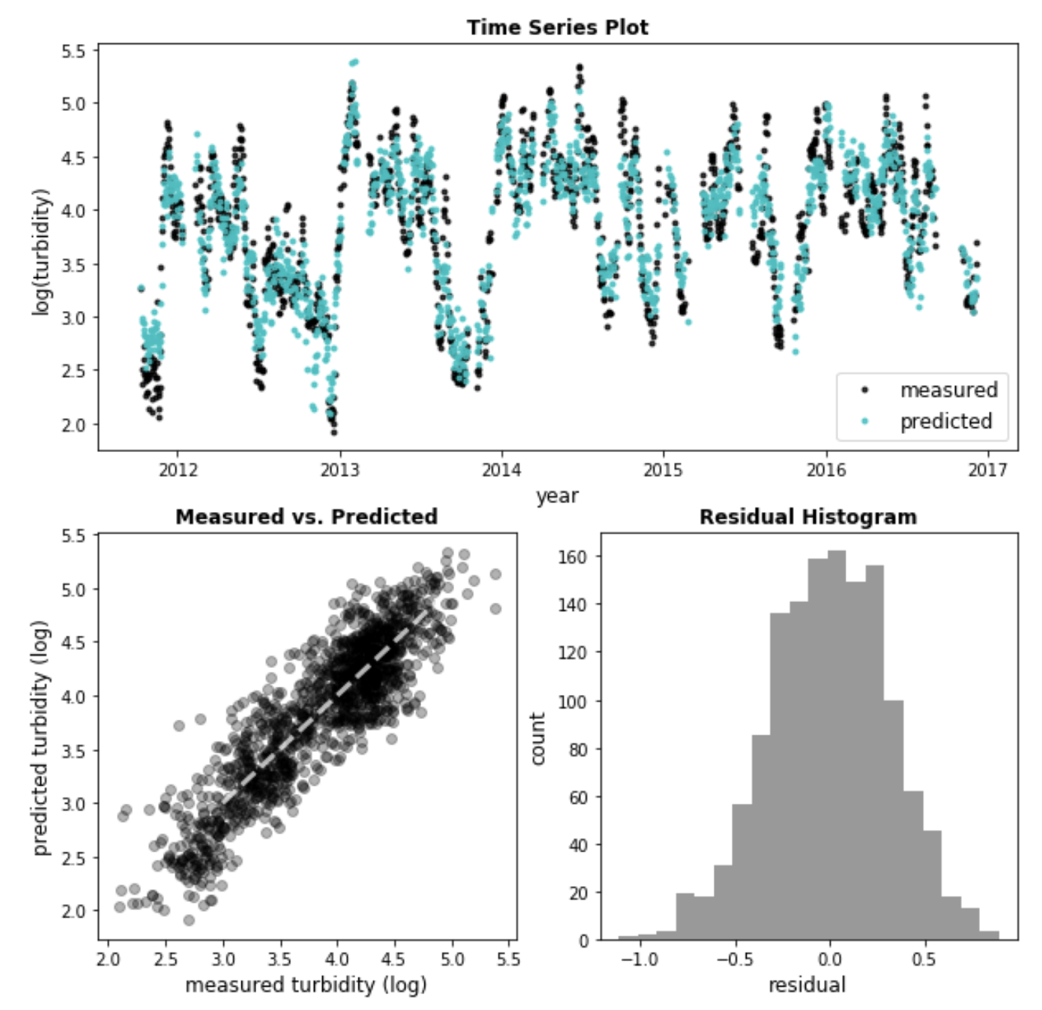
Downloaded data was then cleaned by removing missing values. The result was 113 upstream stations with discharge or stage data (independent variables) and 1 downsteam turbidity data (dependent variable) for 6 years (2011-2017). Sample histogram plots show that distributions are mostly positively skewd, therefore a log transformation was applied to all variables.

Basic OLS

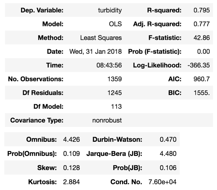
As a first attempt, an Ordinary Least Square (OLS) regression was fitted using all 113 stations as features.

Diagnose statistics: the basic OLS model gives an R2 of 0.79 and a probability of F-statistics below 0.005 - it means the relationship is quite significant. Look further into the residuals, Omnibus and JB test are in the safe zone (p>0.05), the normal distirbution hypothesis could be kept. Although Durbin-Waston test shows autocorrelation in the residuals (<1.5) - not uncommon for time series.

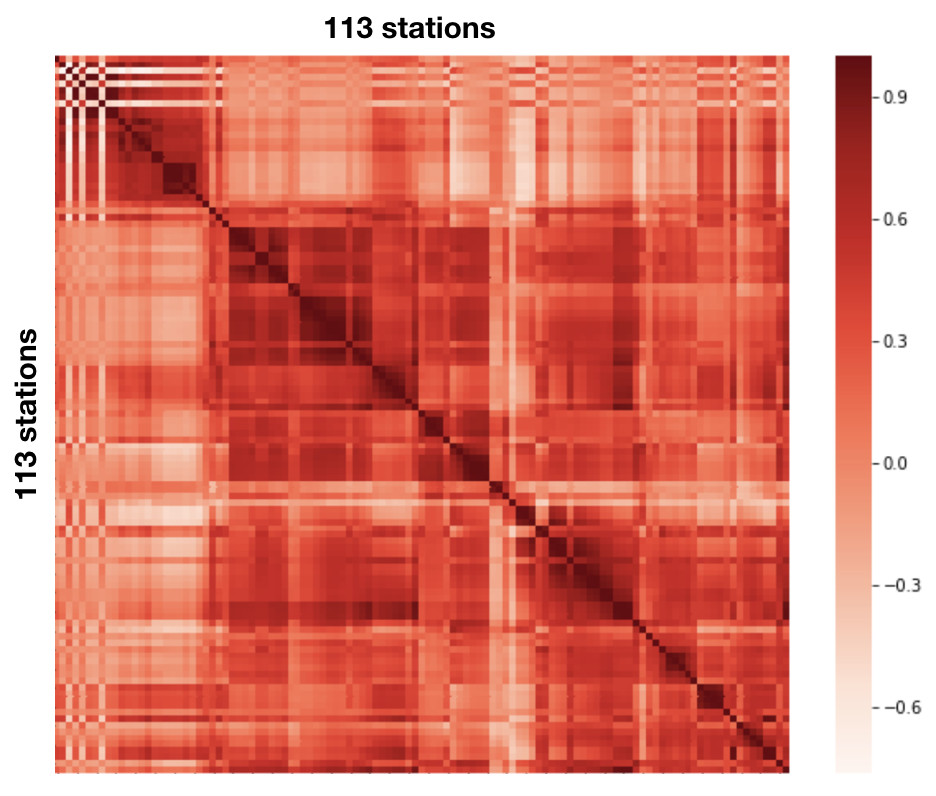
Multicollinearity: many of the stations are not far from each other on the same tributary, so the multicollinearity between feautures are quite significant, i.e., the discharge/stage data are highly correlated. The heat map below visualize the situation:

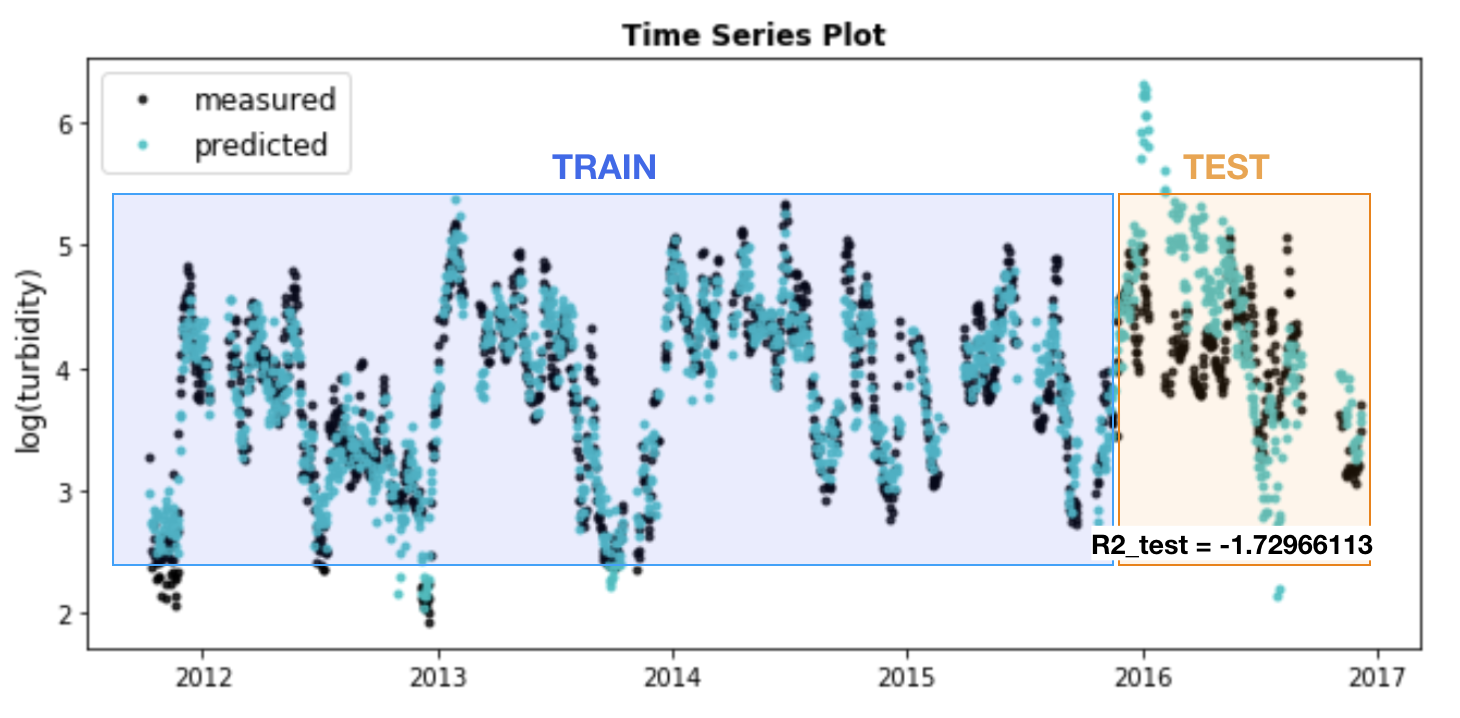
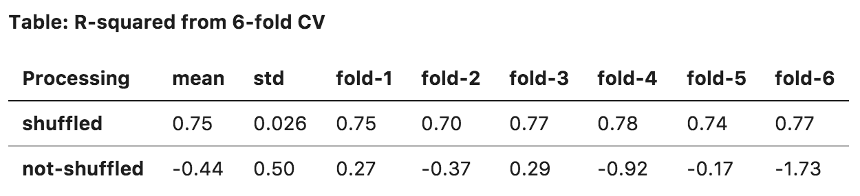
Cross-Validation: here things got interesting. A 6-fold cross-validation was applied to the basic OLS model. It turned out that whether the rows are shuffled made a big impact. Remember that all data are time series, therefore splitting unshuffled data is equivalently training on a 5-year timeseries, and test on the 1-year timeseries that was left out (see figure below). In the case of shuffled data, it essentially allowed training set to randomly sample through the whole 6-year duration, and the model was able to learn for period of time.

Regularization

For the next step, regularization was applied to remove multicollinearity and excess features. This helps to generalize the model and improve out-of-sample performance.

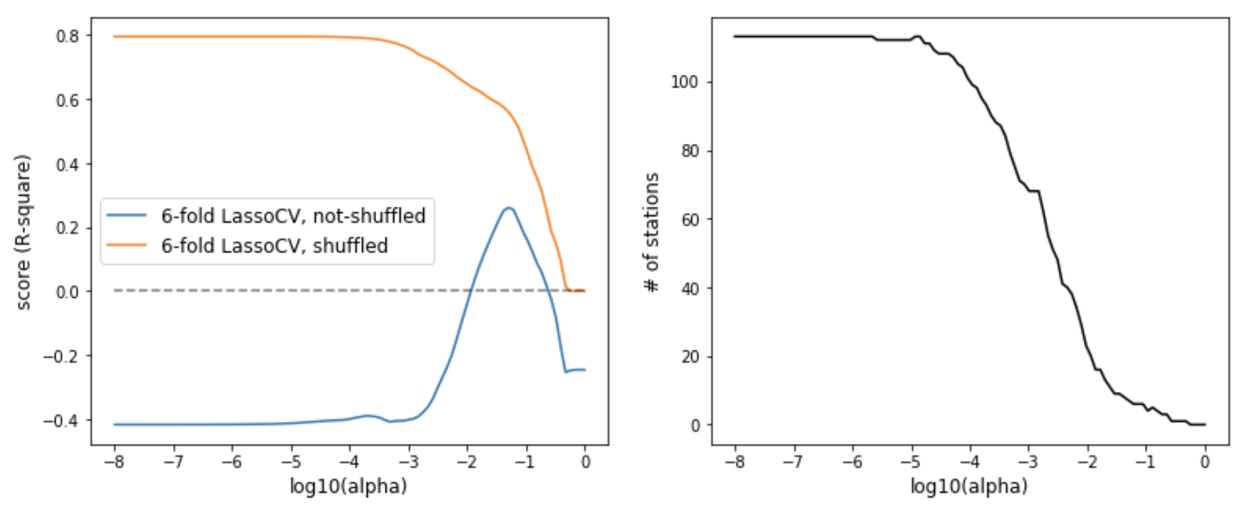
Lasso: my default choice was Lasso regularization, for its ability to quickly eliminate features. Lasso essentially puts a L1-norm penalty on coefficients. I combined Lasso with the 6-fold cross-validation described above. The strengh of penalty (alpha) varied evenly in log space from 1e-8 to 1.0. Again, shuffling the data made a big difference. While shuffled score remained high until big penalty, unshuffled CV remained low but had a small peak of R2 ~= 0.26 with alpha ~= 0.05.

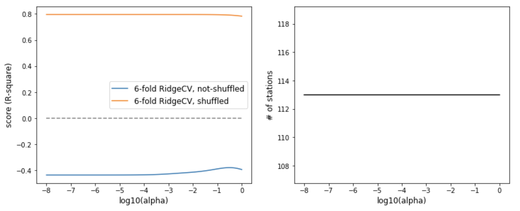
Ridge/ElasticNet out of curiosity, I also experimented with Ridge and ElasticNet. Seems that Lasso is still the better choice for this particular problem.

Recursive feature selection

Sklearn has a built-in function for feature selection RFE. By specifying the number of features to keep, the function return the best fit by recursively testing a subset of the features of the given size. The scoring method is 6-fold cross-validation with shuffled data. Note the plunge of R-squared score around 15 features.

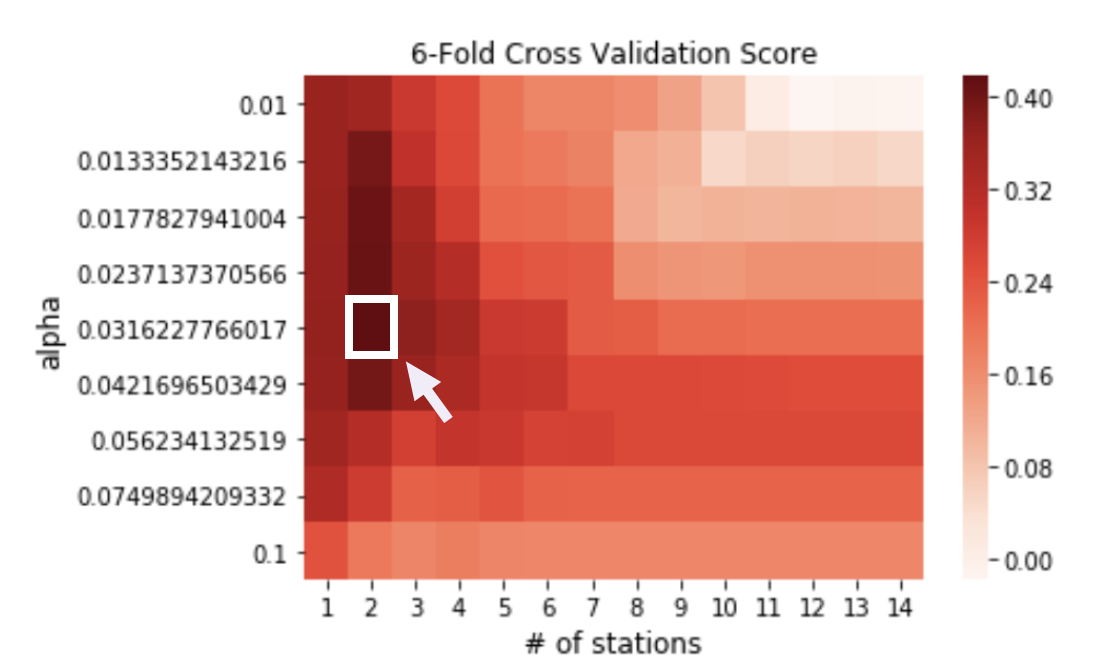
A grid search is then implemented by combining a range of feature numbers for RFE (1-15) and a range of alpha values for Lasso CV (1e-2 to 1e-1, 9 values total). Results showed a peak of R2 (~=0.41) with 2 stations and alpha around 0.032.

Conclusion and future directions

• Relationships learnt from past years do not extrapolate well into the future. However, they are good at filling missing values (R2>0.7);
• For the purpose of sediment forecast, the best way is to fit a model is using most recent data (1~2 years);
• Predictions are likely to benefit from information beyond instantaneous measurements, therefore timeseries analysis should be considered to account for temporal patterns;

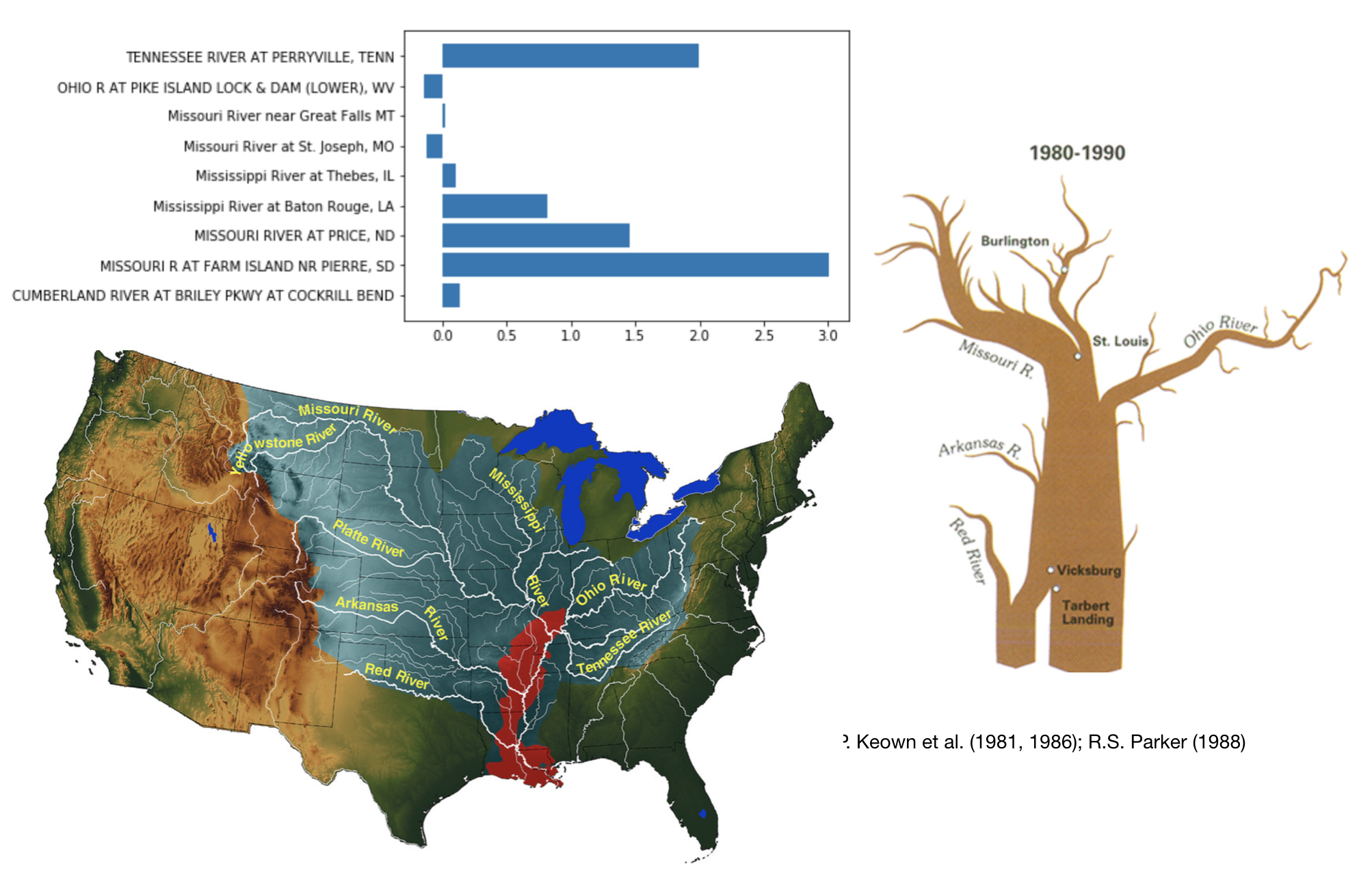
• Last but not least, here are a list of upstream stations that with the most significant contribution to the downstream sediment concentration based on the linear regression model:

  1.99 ‘TENNESSEE RIVER AT PERRYVILLE, TENN’
  1.46, ‘MISSOURI RIVER AT PRICE, ND’
  2.98, ‘MISSOURI R AT FARM ISLAND NR PIERRE, SD’
  0.81, ‘Mississippi River at Baton Rouge, LA’

Interestingly, the relative weights of their coefficients roughly resembles previous studies on the major sediment sources in the Mississippi River.

Final Thoughts

Despite not being considered an advanced technique in the family of machine learning, linear regression still has in depth sciences going into it. Building a really good linear regression model deserves more credits for all the efforts involved.

RETURN TO BLOG